In class we estimate autoregressive models of ln(real GDP). Case 3 is an AR(1), Case 4 is an I(1), and Case 5 is an ARI(1,1).
The I indicates the special case where the coefficient on a lagged dependent variable (sometimes with a little algebra and the Engle-Granger Representation Theorem) is restricted to equal one. You don’t get a stochastic trend without that restriction. So Case 4 is a restriction on Case 3, and Case 5 could be thought of as an AR(2) with one of those restricted.
TS asked after class the other day if these sort of models are used for serious forecasting. My response was that, after removing a lot of details, all serious economic and financial forecasting models have AR(p) and ARI(p,1) processes at their core.
Using any of these is a craft, and one of the things you learn is that while they can do pretty good forecasts in the short-run, their long-run forecasts are sort of uninteresting. They’re not necessarily wrong, but they may not say much.
The reason for this is those lags. They contain all the information that makes the forecasts work. This works for forecasting one period ahead (t+1) because you have the data from time t to use in your model. But what if you want to forecast t+2? Where do you get the data from t+1 for the lags? One thing you can do is use your forecast of t+1 that you made at t as an input to make your forecast for t+2. This works OK. But the forecast made at t of t+1 is missing whatever shocks do happen at t+1 to make that period interesting, so the forecasts for t+2 tend to be a little plain and less volatile. The further you go into the future, the worse that problem gets.
The end result of this is that forecasts from AR(p) and ARI(p,1) models tend to converge to the average after a few periods.
Now combine that with the idea of the stochastic trend that you get from the I(1) part of those models. This is saying that there is no central tendency for the trend to return to. It’s always there, but it comes off the most recent data point you’re at. You can be above or below it in the short-run, but the best thing we can say is that in the long-run you’ll settle down to that particular stochastic trend. If there’s a shock next period, your stochastic trend will shift, but the new forecast is that you’ll still settle down to that new one.
So, check out these 10-year Treasury Bond rate forecasts:
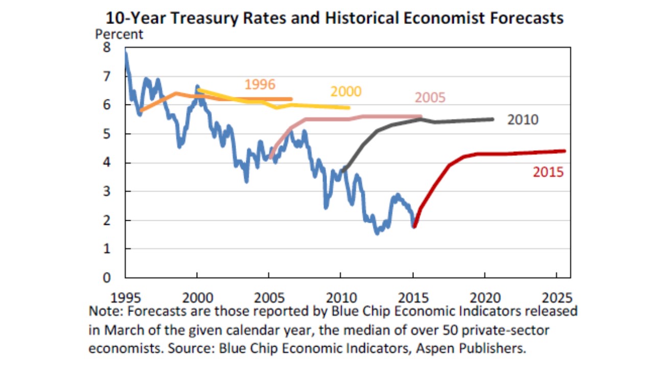
These are collected from Blue Chip, which surveys the most popular economic forecasters, who are (no doubt) using an ARI(p,1) model for these.†
What each colored curve is showing is the forecast from a particular point in time. They all wobble a bit in the short-run before converging to a flat line in the long-run. This is just an example. When you see this behavior in future publications, you know where it’s coming from.
You can check out the source post entitled “Losing Interest” at the Lawrence Economics Blog, but the whole thing is not required.
† Technically, the rates themselves are probably not an ARI(p,1). But rates are formed as a ratio of coupon payments and total amount borrowed, both of which do follow that sort of process.
No comments:
Post a Comment